# Load packages and function
library(tidyverse)
library(here)
library(tmap)
library(showtext)
library(scales)
library(ggalluvial)
library(geobr)
library(sf)
source(here("R","clean.R"))
# Read data
mining_amazon <- read.csv(here("data", "mining_amazon.csv"))
mining_cerrado <- read.csv(here("data", "mining_cerrado.csv"))
mining_forest <- read.csv(here("data", "mining_mata_atlantica.csv"))
# Apply function to all biome datasets
mining_amazon <- clean_df(mining_amazon) %>% mutate(Biome = "Amazon")
mining_cerrado <- clean_df(mining_cerrado) %>% mutate(Biome = "Cerrado")
mining_forest <- clean_df(mining_forest) %>% mutate(Biome = "Atlantic Forest")
# Combine the rows from all dataframes and create column that sum all the mining area
total_mining <- bind_rows(
mining_amazon,
mining_cerrado,
mining_forest
) %>%
mutate(Total = rowSums(across(-c(Ano, Biome)), na.rm = TRUE))
# Transform to long format
mining_long <- total_mining %>%
select(-ends_with(".1")) %>% # Remove all .1 columns
pivot_longer(
cols = -c(Ano, Biome, Total),
names_to = "Mineral",
values_to = "Area") %>%
mutate(
Mineral = case_match(
Mineral,
"Ouro" ~ "Gold",
"Ferro" ~ "Iron",
"Alumínio" ~ "Aluminum",
"Estanho" ~ "Tin",
"Carvão.mineral" ~ "Coal",
"Cobre" ~ "Copper",
"Calcário" ~ "Limestone",
"Minerais.de.Classe.2" ~ "Class 2",
"Rochas.ornamentais" ~ "Ornamental rocks",
"Nióbio" ~ "Niobium",
"Manganês" ~ "Manganese",
.default = Mineral
)
) %>% drop_na(Area)
# Filter data to 2024 and calculate percentage
data_2024 <- mining_long %>%
filter(Ano == 2024) %>%
group_by(Biome, Mineral) %>%
summarise(Area = sum(Area, na.rm = TRUE), .groups = "drop") %>%
group_by(Biome) %>%
mutate(
Percentage = Area / sum(Area) * 100,
Mineral = if_else(
dense_rank(desc(Area)) <= 5,
Mineral,
"Other"
)
) %>%
group_by(Biome, Mineral) %>%
summarise(Percentage = sum(Percentage), .groups = "drop") %>%
mutate(
Biome = factor(Biome, levels = c("Amazon", "Atlantic Forest", "Cerrado"))
)
# Prepare data for 1985 and 2024 comparison
sankey_data <- mining_long %>%
filter(Ano %in% c(1985, 2024), !is.na(Area), Area > 0) %>%
group_by(Ano, Mineral) %>%
summarise(Area = sum(Area, na.rm = TRUE), .groups = "drop") %>%
group_by(Ano) %>%
mutate(
Percentage = Area / sum(Area) * 100,
Mineral = if_else(
dense_rank(desc(Area)) <= 8,
Mineral,
"Other"
)
) %>%
group_by(Ano, Mineral) %>%
summarise(
Area = sum(Area, na.rm = TRUE),
Percentage = sum(Percentage),
.groups = "drop"
)
# Define biome color palette
biome_colors <- c(
"Amazon" = "#758E4F",
"Atlantic Forest" = "#33658A",
"Cerrado" = "#B37761"
)
# Define mineral color palette for pit mining
mineral_colors <- c(
"Gold" = "#DABA7E",
"Iron" = "#AB6062",
"Aluminum" = "#5E6284",
"Tin" = "#D8CCB5",
"Coal" = "#2F4F4F",
"Copper" = "#B87333",
"Limestone" = "#BFC6C3",
"Class 2" = "#859D8B",
"Ornamental rocks" = "#8B7355",
"Niobium" = "#556F7A",
"Other" = "#695152"
)
# Plot 1: Mining by year and biome
total_mining <- total_mining %>%
mutate(Biome = factor(Biome, levels = c("Cerrado", "Atlantic Forest", "Amazon")))
plot1 <- ggplot(total_mining, aes(x = Ano, y = Total, fill = Biome)) +
geom_area() +
facet_wrap(~Biome) +
scale_fill_manual(values = biome_colors) +
scale_y_continuous(labels = scales::comma_format()) +
theme_minimal() +
labs(
x = "Year",
y = "Mining Area (hectares)",
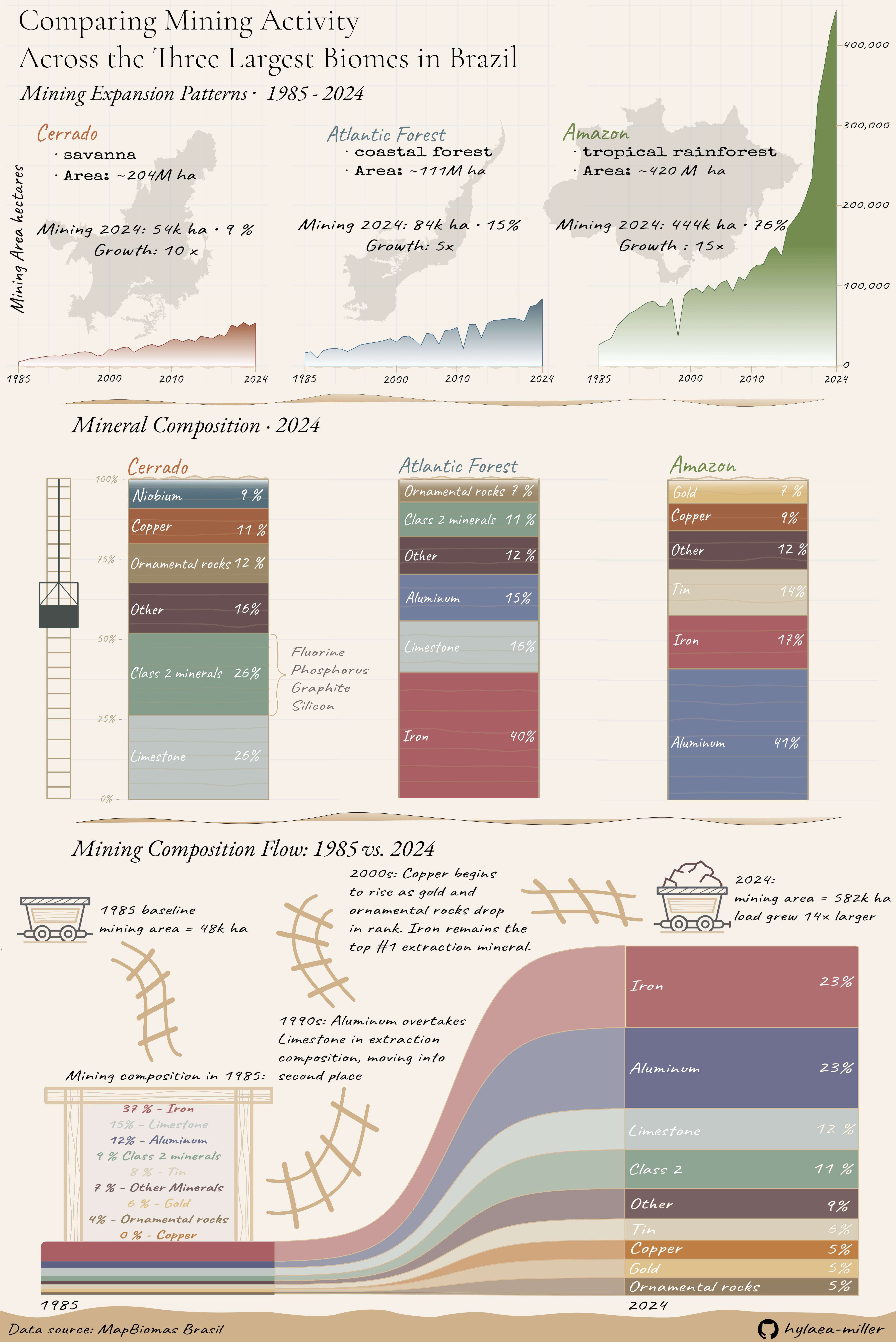
title = "Mining Expansion Patterns Across Brazil's Three Largest Biomes (1985-2024)",
subtitle = "Amazon shows steep growth post-2015, while Atlantic Forest and Cerrado grew more steadily"
) +
theme(legend.position = "none",
plot.title = element_text(
face = "bold",
size = rel(1.5),
lineheight = 1.3,
color = "#2C3E50"
),
plot.subtitle = element_text(
size = rel(1.2),
color="#7F8C8D",
),
plot.caption = element_text(
size = rel(1.3),
color = "#7F8C8D",
hjust = 0,
face = "italic",
margin = margin(t = 10)
),
axis.text = element_text(size = rel(1.3)),
axis.title.x = element_text(
size = rel(1.3),
margin = margin(t = 15)),
axis.title.y = element_text(
size = rel(1.3),
margin = margin(r = 10))
)
# Create a function to generate the mining‑composition plot for a selected biome
plot_biome <- function(biome_name) {
data_2024 %>%
filter(Biome == biome_name) %>%
mutate(Mineral = fct_reorder(Mineral, Percentage)) %>%
ggplot(aes(x = "", y = Percentage, fill = Mineral)) +
geom_col(width = 0.6) +
scale_fill_manual(values = mineral_colors) +
scale_y_continuous(labels = percent_format(scale = 1), expand = c(0, 0)) +
labs(title = biome_name, x = NULL, y = "Percentage of Mining Area") +
theme_minimal() +
theme(
legend.position = "none",
plot.title = element_text( face = "bold", size = rel(1.7), color = "#2C3E50"),
axis.text = element_text(size = rel(1.5), color = "#34495E"),
axis.title.x = element_text(size = rel(1.5), face = "bold", color = "#34495E")
)
}
plot2_cerrado <- plot_biome("Cerrado")
plot2_atlantic <- plot_biome("Atlantic Forest")
plot2_amazon <- plot_biome("Amazon")
# Adjust data to the sankey plot
sankey_data <- sankey_data %>%
complete(
Ano,
Mineral,
fill = list(Area = 0)
)
# Order minerals by 2024 (descending)
mineral_order_2024 <- sankey_data %>%
filter(Ano == 2024) %>%
arrange(desc(Area)) %>%
pull(Mineral)
# Order minerals by 1985 (descending)
mineral_order_1985 <- sankey_data %>%
filter(Ano == 1985) %>%
arrange(desc(Area)) %>%
pull(Mineral)
sankey_data <- sankey_data %>%
mutate(
Mineral = factor(Mineral, levels = mineral_order_1985)
)
# Plot Sankey diagram
plot3 <- ggplot(
sankey_data,
aes(
x = factor(Ano),
y = Area,
stratum = Mineral,
alluvium = Mineral
)) +
geom_flow(
aes(fill = Mineral),
alpha = 0.6,
curve_type = "sigmoid",
width = 0.4 ) +
geom_stratum(
aes(fill = Mineral),
alpha = 0.9,
width = 0.4
) +
geom_text(
stat = "stratum",
aes(
label = if_else(
as.integer(as.character(Ano)) == 2024,
paste0(Mineral, "\n", round(Percentage, 1), "%"),
""
)),
color = "white",
size = 3.5,
fontface = "bold"
) +
scale_fill_manual(values = mineral_colors, drop = FALSE) +
labs(title = "Changes in Brazil's Mining Composition, 1985–2024") +
theme_void() +
theme(
axis.text.x = element_text(),
legend.position = "none",
plot.title = element_text(
face = "bold",
size = 18,
hjust = 0.5,
color = "#2C3E50",
margin = margin(b = 5, t = 20) ),
plot.caption = element_text(
size = rel(1.5),
color = "#7F8C8D",
hjust = 0,
face = "italic",
margin = margin(t = 10)))
# Read Brazil biomes data
biomes <- read_biomes(year = 2019)
# Plot the biomes
biomes <- plot(st_geometry(biomes))